

Table of Contents
Motivation
Among the integration methods introduced in Integration, the Monte Carlo method is the most powerful one in high dimensions. The term Monte Carlo is used as a synonym for the use of pseudo-random numbers. Markov chains are a particular class of Monte Carlo algorithms designed to generate correlated samples from an arbitrary distribution. The central workhorse in BAT is an adaptive Markov chain Monte Carlo (MCMC) implementation based on the Metropolis algorithm. It allows users to marginalize a posterior without requiring manual tuning of algorithm parameters. In complicated cases, tweaking the parameters can substantially increase the efficiency, so BAT gives users full access to all tuning parameters.
Foundations
Monte Carlo integration
We begin with the fundamental Monte Carlo principle. Suppose we have a posterior probability density \(P(\vecth|D)\), often called the target density, and an arbitrary function \(f(\vecth)\) with finite expectation value under \(P\)
\begin{align} \label{eq:mc-expect} E_P[ f ] = \int \rmdx{ \vecth} P(\vecth|D) f(\vecth) < \infty . \end{align}
Then a set of draws \(\{ \vecth_i:i=1 \dots N \}\) from the density \(P\), that is \(\vecth_i \sim P\), is enough to estimate the expectation value. Specifically, the integral can be replaced by the estimator (distinguished by the symbol \(\widehat{\phantom{a}}\))
\begin{align} \label{eq:mc-expect-discrete} \boxed{ \widehat{E_P[f]} \approx \frac{1}{N} \sum_{i=1}^{N} f(\vecth_i), \; \vecth \sim P } \end{align}
As \(N \to \infty\), the estimate converges almost surely at a rate \(\propto 1/\sqrt{N}\) by the strong law of large numbers if \(\int \rmdx{ \vecth} P(\vecth|D) f^2(\vecth) < \infty\) [11] . This is true for independent samples from the target but also for correlated samples. The only thing that changes is the increased variance of the estimator due to correlation.

How does this relate to Bayesian inference? Upon applying Bayes’ theorem to real-life problems, one usually has to marginalize over several parameters, and this can usually not be done analytically, hence one has to resort to numerical techniques. In low dimensions, say \(d \le 2\), quadrature and other grid-based methods are fast and accurate, but as \(d\) increases, these methods generically suffer from the curse of dimensionality. The number of function evaluations grows exponentially as \(\order{m^d}\), where \(m\) is the number of grid points in one dimension. Though less accurate in few dimensions, Monte Carlo — i.e., random-number based — methods are the first choice in \(d \gtrsim 3\) because the computational complexity is (at least in principle) independent of \(d\). Which function \(f\) is of interest to us? For example when integrating over all but the first dimension of \(\vecth\), the marginal posterior probability that \(\theta_1\) is in \([a,b)\) can be estimated as
\[ \label{eq:disc-marg} P(a \le \theta_1 \le b|D) \approx \frac{1}{N} \sum_{i=1}^{N} \mathbf{1}_{\theta_1 \in [a,b)} (\vecth_i) \, \]
with the indicator function
\[ \label{eq:indicator-fct} \mathbf{1}_{\theta_1 \in [a,b)} (\vecth) = \begin{cases} 1, \theta_1 \in [a,b) \\ 0, {\rm else} \end{cases} \]
This follows immediately from the Monte Carlo principle with \(f(\vecth) = \mathbf{1}_{\theta_1 \in [a,b)}(\vecth)\). The major simplification arises as we perform the integral over \(d-1\) dimensions simply by ignoring these dimensions in the indicator function. If the parameter range of \(\theta_1\) is partitioned into bins, then the above holds in every bin, and defines the histogram approximation to \(P(\theta_1|D)\). In exact analogy, the 2D histogram approximation is computed from the samples for 2D bins in the indicator function. For understanding and presenting the results of Bayesian parameter inference, the set of 1D and 2D marginal distributions is the primary goal. Given samples from the full posterior, we have immediate access to all marginal distributions at once; i.e., there is no need for separate integration to obtain for example \(P(\theta_1|D)\) and \(P(\theta_2|D)\). This is a major benefit of the Monte Carlo method in conducting Bayesian inference.
Metropolis algorithm
The key ingredient in BAT is an implementation of the Metropolis algorithm to create a Markov chain; i.e. a sequence of (correlated) samples from the posterior. We use the shorthand MCMC for Markov chain Monte Carlo.
Efficient MCMC algorithms are the topic of past and current research. This section is a concise overview of the general idea and the algorithms available in BAT. For a broader overview, we refer the reader to the abundant literature; e.g., [11] [2] .
In BAT, there are several variants of the random-walk Metropolis Hastings algorithm available. The basic idea is captured in the 2D example plot. Given an initial point \(\vecth_0\), the Metropolis algorithm produces a sample in each iteration \(t=1 \dots N \) as follows:
- Propose a new point \(\tilde{\vecth}\)
- Generate a number u from the uniform distribution on [0,1]
- Set \(\vecth_{t} = \tilde{\vecth}\) if \( u < \frac{P(\tilde{\vecth} \cond D)}{P(\vecth_{t-1} \cond D)}\)
- Else stay, \(\vecth_t = \vecth_{t-1}\)
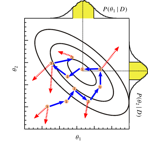
In the example plot, the chain begins in the lower left corner. Rejected moves are indicated by the dashed arrow, accepted moves are indicated by the solid arrow. The circled number is the number of iterations the chain stays at a given point \(\vecth = (\theta_1, \theta_2)\).
In each iteration \(t\), one updates the estimate of the 1D marginal distribution \(P(\theta_1 | D)\) by adding the first coordinate of \(\vecth_t\) to a histogram. Repeat this for all other coordinates to update the other \((d-1)\) 1D marginals. And redo it for all pairs of coordinates to estimate the 2D marginals.
As a concrete example, suppose the chain has 5 iterations in 2D:
| \(t\) | \(\vecth_t\) |
|---|---|
| 1 | \((1.1, 2.3)\) |
| 2 | \((1.1, 2.3)\) |
| 3 | \((3.8, 1.8)\) |
| 4 | \((2.4, 5.2)\) |
| 5 | \((1.8, 4.2)\) |
Let us choose a histogram to approximate the 1D marginal posterior for \(\theta_1\) with five bins from \([n, n+1)\) for \(n=0 \dots 4\) such that the right edge of the bin is not included. Up to \(t=5\), the histogram is
| \(n\) | weight |
|---|---|
| 0 | 0 |
| 1 | 3 |
| 2 | 1 |
| 3 | 1 |
| 4 | 0 |
In the end, we usually normalize the histogram so it estimates a proper probability density that integrates to 1.
Convergence
Since samples are not independent, the initial point has some effect on Markov chain output. The asymptotic results guarantee that, under certain conditions (see [11] or [2]) a chain of infinite length is independent of the initial point. In practice, we can only generate a finite number of points so a decision has to be made when the chain has run long enough. One helpful criterion is to run multiple chains from different initial positions and to declare convergence if the chains mixed; i.e. explore the same region of parameter space. Then the chains have forgotten their initial point.
Non-convergence is a problem that can have many causes including simple bugs in implementing the posterior. But there are properly implemented posteriors for which a Markov chain has difficulties to explore the parameter space efficiently, for example because of strong correlation, degeneracies, or multiple well separated modes.
Implementation in BAT
Implementing the Metropolis algorithm, one has to decide on how to propose a new point based on the current point, that is one needs the proposal function \(q(\tilde{\vecth} \cond \vecth_t, \xi)\) with adjustable parameters \(\xi\). The main difference between MCMC algorithms is typically given by different choices of \(q\). The Metropolis algorithm doesn't specify which \(q\) to choose, so we can and have to select a function \(q\) and tune \(\xi\) according to our needs.
In BAT, the proposal is symmetric around the current point
\begin{align} q(\tilde{\vecth} \cond \vecth_t, \xi) = q(\vecth_t \cond \tilde{\vecth}, \xi). \end{align}
The Markov property implies that the proposal may only depend on the current point \(\vecth_t\) and not on any previous point. If the value of \(\xi\) is set based on a past sequence of iterations of the chain, we need two stages of sampling in BAT, the prerun and the main run. In the prerun, the chain is run and periodically \(\xi\) is updated based on the past iterations. In contrast, \(\xi\) is kept fixed in the main run to have a proper Markov chain.
Proposal functions
BAT offers two kinds of proposal function termed factorized and multivariate. The general form is either a Gaussian or Student's t distribution. In the factorized case, the joint distribution is a product of 1D distributions. In the multivariate case, a dense covariance matrix is used that allows correlated proposals. In either case, the default is Student's t distribution with one degree of freedom (dof); i.e., a Cauchy distribution. Select the proposal like this:
Multivariate proposal
- Since
- Introduced and set as the default in v1.0
Changing all \(d\) parameters at once within one iteration is an all-or-nothing approach. If the proposed move is accepted, all parameters have changed for the price of a single evaluation of the posterior. If the move is rejected, the new point is identical to the old point and the chain does not explore the parameter space.
We implement the adaptive algorithm by Haario et al. [6], [15]. In brief, the proposal is a multivariate Gaussian or Student's t distribution whose covariance is learned from the covariance of samples in the prerun. An overall scale factor is tuned to force the acceptance rate into a certain range.
the multivariate normal distribution
\begin{equation} \label{eq:multivar-normal} \mathcal{N}(\vecth | \vecmu, \matsig) = \frac{1}{(2\pi)^{d/2}} \left|\matsig\right|^{-1/2} \exp(-\frac{1}{2} (\vecth - \vecmu)^T \matsig^{-1} (\vecth - \vecmu) ) \end{equation}
or the multivariate Student's t distribution
\begin{equation} \label{eq:multivar-student} \mathcal{T} (\vecth | \vecmu, \matsig, \nu) = \frac{\Gamma( (\nu + d) / 2 )}{\Gamma(\nu / 2) (\pi \nu)^{d/2}} \left|\matsig\right|^{-1/2} ( 1 + \frac{1}{\nu}(\vecth - \vecmu)^T \matsig^{-1} (\vecth - \vecmu) )^{-(\nu + d)/2} \end{equation}
can adapt in such a way as to efficiently generate samples from essentially any smooth, unimodal distribution. The parameter \(\nu\), the degree of freedom, controls the ``fatness'' of the tails of \(\mathcal{T}\); the covariance of \(\mathcal{T}\) is related to the scale matrix \(\matsig\) as \(\frac{\nu}{\nu - 2} \times \matsig\) for \(\nu > 2\), while \(\matsig\) is the covariance of \(\mathcal{N}\). Hence for finite \(\nu\), \(\mathcal{T}\) has fatter tails than \(\mathcal{N}\), and for \(\nu \to \infty\), \(\mathcal{T}(\vecth | \vecmu, \matsig, \nu) \to \mathcal{N}(\vecth | \vecmu, \matsig)\).
Before delving into the details, let us clarify at least qualitatively what we mean by an efficient proposal. Our requirements are
- that it allow to sample from the entire target support in finite time,
- that it resolve small and large scale features of the target,
- and that it lead to a Markov chain quickly reaching the asymptotic regime.
An important characteristic of Markov chains is the acceptance rate \(\alpha\), the ratio of accepted proposal points versus the total length of the chain. We argue that there exists an optimal \(\alpha\) for a given target and proposal. If \(\alpha = 0\), the chain is stuck and does not explore the state space at all. On the contrary, suppose \(\alpha = 1\) and the target distribution is not globally uniform, then the chain explores only a tiny volume where the target distribution changes very little. So for some \(\alpha \in (0,1)\), the chains explore the state space well.
How should the proposal function be adapted? After a chunk of \(N_{\rm update}\) iterations, we change two things. First, in order to propose points according to the correlation present in the target density, the proposal scale matrix \(\matsig\) is updated based on the sample covariance of the last \(n\) iterations. Second, \(\matsig\) is multiplied with a scale factor \(c\) that governs the range of the proposal. \(c\) is tuned to force the acceptance rate to lie in a region of \(0.15 \le \alpha \le 0.35\). The \(\alpha\) range is based on empirical evidence and the following fact: for a multivariate normal proposal function, the optimal \(\alpha\) for a normal target density is \(0.234\), and the optimal scale factor is \(c = 2.38^2/d\) as the dimensionality \(d\) approaches \(\infty\) and the chain is in the stationary regime [12] . We fix the proposal after a certain number of adaptations, and then collect samples for the final inference step. However, if the Gaussian proposal function is adapted indefinitely, the Markov property is lost, but the chain and the empirical averages of the integrals still converge under mild conditions [6].
The efficiency can be enhanced significantly with good initial guesses for \(c\) and \(\matsig\). We use a subscript \(t\) to denote the status after \(t\) updates. It is often possible to extract an estimate of the target covariance by running a mode finder like MINUIT that yields the covariance matrix at the mode as a by product of optimization. In the case of a degenerate target density, MINUIT necessarily fails, as the gradient is not defined. In such cases, one can still provide an estimate as
\begin{equation} \label{eq:sigma-initial} \matsig^0 = \diag ( \sigma_1^2, \sigma_2^2, \dots, \sigma_d^2) \end{equation}
where \(\sigma_i^2\) is the prior variance of the \(i\)-th parameter. The updated value of \(\matsig\) in step \(t\) is
\begin{equation} \label{eq:sigma-update} \matsig^t = (1 - a^t) \matsig^{t-1} + a^t \boldsymbol{S}^t \end{equation}
where \(\boldsymbol{S}^t\) is the sample covariance of the points in chunk \(t\) and its element in row \(m\) and column \(n\) is computed as
\begin{equation} \label{eq:sample-cov} (\boldsymbol{S}^t)_{mn} = \frac{1}{N_{\rm update}-1} \sum_{i=(t-1) \cdot N_{\rm update}}^{t \cdot N_{\rm update}} ( (\vecth^i)_m - \widehat{E_P[(\vecth)_m]} ) ((\vecth^i)_n - \widehat{E_P[(\vecth)_n]} ) \end{equation}
The weight \(a^t = 1/t^{\lambda}, \lambda \in [0,1]\) is chosen to make for a smooth transition from the initial guess to the eventual target covariance, the implied cooling is needed for the ergodicity of the chain if the proposal is not fixed at some point [6]. One uses a fixed value of \(\lambda\), and the particular value has an effect on the efficiency, but the effect is generally not dramatic; in this work, we set \(\lambda=0.5\) [15].
We adjust the scale factor \(c\) as described in the pseudocode shown below. The introduction of a minimum and maximum scale factor is a safeguard against bugs in the implementation. The only example we can think of that would result in large scale factors is that of sampling from a uniform distribution over a very large volume. All proposed points would be in the volume, and accepted, so \(\alpha \equiv 1\), irrespective of \(c\). All other cases that we encountered where \(c > c_{max}\) hinted at errors in the code that performs the update of the proposal.
- See also
BCEngineMCMC::SetMultivariateCovarianceUpdateLambda,BCEngineMCMC::SetMultivariateEpsilon,BCEngineMCMC::SetMultivariateScaleMultiplier
Factorized proposal
- Since
- Factorized was the default and only choice prior to v1.0 and continues to be available using
BCEngineMCMC::SetProposeMultivariate(false)
The factorized proposal in \(d\) dimensions is a product of 1D proposals.
We sequentially vary one parameter at a time and complete one iteration of the chain once a new point has been proposed in every direction. This means the chain attempts to perform a sequence of axis-aligned moves in one iteration.
Each 1D proposal is a Cauchy or Breit-Wigner function centered on the current point. The scale parameter is adapted in the prerun to achieve an acceptance rate in a given range that can be adjusted by the user. Note that there is a separate scale parameter in every dimension.
This means the posterior is called \(d\) times in every iteration. Since the acceptance rate is typically different from zero or one, the factorized proposal typically generates a new point in every iteration that differs from the previous point in some but not all dimensions.
Comparison
Comparing the factorized proposal to the multivariate proposal, we generally recommend the multivariate for most purposes.
Use the factorized proposal if you can speed up the computation of the posterior if you know that some parameters did not change. This can be useful if the computation is expensive if some but not all parameters change.
Prerun
During the prerun, the proposal is updated. BAT considers three criteria to decide when to end the prerun. The prerun takes some minimum number of iterations and is stopped no matter what if the maximum number of prerun iterations is reached. In between, the prerun terminates if the efficiency and the \(R\) value checks are ok. To perform the prerun manually, do
In most cases this is not needed, because BCModel::MarginalizeAll calls BCEngineMCMC::Metropolis, which will take care of the prerun and the main run and all the data handling associated with it. To force a prerun to be run again, perhaps after it failed and some settings have been adjusted, do:
Efficiency
The efficiency, or acceptance rate, is the ratio of the accepted over the total number proposal moves. A small efficiency means the chain rarely moves but may then make a large move. A large efficiency means the chain explores well locally but may take a long time to explore the entire region of high probability. Optimality results exists only for very special cases: Roberts and Rosenthal showed that for a Gaussian target with \(d\) independent components and a Gaussian proposal, the optimal target efficiency is 23.4 % for \(d \geq 5\) is but should be larger for small \(d\); e.g., 44 % is best in one dimension [13] . Based on our experience, we use a default range for the efficiency as \([0.15, 0.35]\).
R value
The R value [4] by Gelman and Rubin quantifies the estimated scale reduction of the uncertainty of an expectation value estimated with the samples if the chain were run infinitely long. Informally, it compares the mean and variance of the expectation value for a single chain with the corresponding results of multiple chains. If the chains mix despite different initial values, then we assume that they are independent of the initial value, the burn-in is over, and the samples produce reliable estimates of quantities of interest. For a single chain, the \(R\) value cannot be computed.
In BAT, we monitor the expectation value of each parameter and declare convergence if all R values are below a threshold. Note that the R values are estimated from batches of samples, and they usually decrease with more iterations but they may also increase, which usually is a clear indication that the chains do not mix, perhaps due to multiple modes that trap the chains.
- See also
BCEngineMCMC::SetRValueParametersCriterionSet the maximum allowed \(R\) value for all parameters. By defition, \(R\) cannot go below 1 except for numerical inaccuracy. Default: 1.1-
BCEngineMCMC::SetCorrectRValueForSamplingVariabilityThe strict definition of \(R\) corrects the sampling variability due finite batch size. Default: false -
BCEngineMCMC::GetRValueParameters\(R\) values are computed during the prerun and they can be retrieved but not set.
Prerun length
Defining convergence automatically based on the efficiency or the \(R\) value is convenient may be too conservative if the user knows a good initial value, a good proposal, etc. For more control the minimum and maximum length of the prerun can be set, too.
- See also
BCEngineMCMC::SetNIterationsPreRunMin,BCEngineMCMC::SetNIterationsPreRunMax-
BCEngineMCMC::SetNIterationsPreRunChecksets the number of iterations between checks
If desired, the statistics can be cleared to remove the effect of a bad initial point with BCEngineMCMC::SetPreRunCheckClear after some set of iterations
For the user's convenience, multiple settings related to precision of the Markov chain can be set at once using BCEngineMCMC::SetPrecision. The default setting is m.SetPrecision(BCEngineMCMC::kMedium).
Main run
In the main run, the proposal is held fixed and each chain is run for BCEngineMCMC::GetNIterationsRun() iterations.
- See also
BCEngineMCMC::SetNIterationsRun
To reduce the correlation between samples, a lag can be introduced to take only every 10th element with BCEngineMCMC::SetNLag.