

Table of Contents
To demonstrate the basic usage of BAT, we will build an example analysis step by step. Step one, naturally, is to install BAT—please refer to the installation chapter in this manual or online. To check if you have BAT installed and accessible, run the following command
bat-config
in your terminal. It should output a usage statement. This program outputs information about your BAT installation:
bat-config Flag | Returned Information |
|---|---|
--prefix | Path to BAT installation |
--version | BAT version identifier |
--libs | Linker flags for compiling code using BAT |
--cflags | C++ compiler flags for compiling code using BAT |
--bindir | Path to BAT binaries directory |
--incdir | Path to BAT include directory |
--libdir | Path to BAT libraries directory |
BAT has a second executable, which creates for you the files necessary to start a basic analysis. We will use this executable to initialize our tutorial project:
bat-project MyTut MyMod
This will create a directory called MyTut that contains
Makefile | a makefile to compile our tutorial project |
runMyTut.cxx | the C++ source to an executable to run our tutorial project |
MyMod.h | the C++ header for our tutorial model MyMod |
MyMod.cxx | the C++ source for our tutorial model MyMod |
If BAT is installed correctly, you can compile and run this project already:
cd MyTut
make
./runMyTut
BAT will issue a series of errors telling you your model has no parameters. Because of course we haven't actually put anything into our model yet. Let's do that.
Defining a model
To define a valid BAT model we must make three additions to the empty model that bat-project has created:
- we must add parameters to our model;
- we must implement a log-likelihood function;
- and we must implement or state our priors.
We will start with a simple model that fits a normal distribution to data, and so has three parameters: the mode ( \(\mu\)) and standard deviation ( \(\sigma\)) of our distribution, and a scaling factor ("height"). We will start with flat priors for all.
How you store and access your data is entirely up to you. For this example, we are going to fit to a binned data set that we store as a ROOT histogram in a private member of our model class. In the header, add to the class
And in the source file, we initialize our fDataHistogram in the constructor; let's also fill it with some random data, which ROOT can do for us using a TF1:
Adding parameters
To add a parameter to a model, call its member function BCModel::AddParameter:
You must indicate a parameter's name and its allowed range, via min and max. Each parameter must be added with a unique name. BAT will also create a "safe version" of the name which removes all non alpha-numeric characters except for the underscore, which is needed for naming of internal storage objects. Each parameter name should also convert to a unique safe name; BAT will complain if this is not the case (and AddParameter will return false).
Optionally, you may add a display name for the parameter and a unit string, both of which are used when BAT creates plots.
The most logical place to add parameters to a model is in its constructor. Let us now edit MyMod.cxx to add our mode, standard deviation, and height parameters inside the constructor:
I have chosen the ranges because I have prior information about the data: the mode of my distribution will be between 5.27 and 5.29; the standard deviation will be between 0.025 and 0.045; and the height will be between 0 and 10. When we provide a prior for a parameter, \(p_0(\lambda)\), the prior BAT uses is
\begin{equation} P_0(\lambda) = \begin{cases} p_0(\lambda),& \text{if } \lambda\in[\lambda_{\text{min}}, \lambda_{\text{max}}],\\ 0,& \text{otherwise.} \end{cases} \end{equation}
So keep mind that the ranges your provide for parameters become part of the prior: BAT will not explore parameter space outside of the range limits you provide.
If you have written the code correctly for adding parameters to your model, your code should compile. BAT will again, though, issue an error if you try to run runMyTut, since we are still missing priors.
Setting prior distributions
There are two ways we may set the prior, \(P_0(\vec\lambda)\) for a parameter point: We can override the function that returns the log a priori probability for a model (BCModel::LogAPrioriProbability) and code anything we can dream of in C++:
In this case, you have to make sure the prior is properly normalized if you wish to compare different models as BAT will not do this for you.
Or we can set individual priors for each parameter, and BAT will multiply them together for us including the proper normalization. If each parameter has a prior that factorizes from all the others, then this is the much better option. In this case, we must not override LogAPrioriProbability. Instead we tell BAT what the factorized prior is for each parameter, by adding a BCPrior object to each parameter after we create it:
We could create a BCConstantPrior object for height just as we created a BCGaussianPrior object for mu and sigma, but BAT has a convenient function that creates one for us.
We can now compile our code and run it. The results will be meaningless, though, since we have yet to define our likelihood.
Defining a likelihood
The heart of our model is the likelihood function—more specifically, since BAT works with the natural logarithm of functions, our log-likelihood function.
Given a histogrammed data set containing numbers of events in each bin, our statistical model is the product of Poisson probabilities for each bin—the probability of the events observed in the bin given the expectation from our model function:
\begin{equation} \mathcal{L}(\vec\lambda) \equiv \prod_{i} \text{Poisson}(n_i|\nu_i), \end{equation}
where \(n_i\) is the number of events in bin \(i\) and \(\nu_i\) is the expected number of events given our model, which we will take as the value of our model function at the center of the bin, \(m_i\),
\begin{equation} \nu_i \equiv f(m_i) = \frac{1}{\sqrt{2\pi}\sigma}\exp{\left(-\frac{(m_i - \mu)^2}{2\sigma^2}\right)}. \end{equation}
Working with the log-likelihood, this transforms into a sum:
\begin{equation} \log\mathcal{L}(\vec\lambda) \equiv \sum_{i} \log\text{Poisson}(n_i|\nu_i). \end{equation}
BAT conveniently has a function to calculate the logarithm of the Poisson distribution (with observed \(x\) and expected \(\lambda\)) for you:
Let us code this into our log-likelihood function:
Looking at the output
Our model class is now ready to go. Let's just make one edit to the runMyTut.cxx file to change our model name from the default "name_me" to something sensible:
We can now compile and run our project:
This will sample from the posterior probability distribution and marginalize the results, saving plots to gaus_mod_plots.pdf. In that file you should see the 1D and 2D marginalizations of our three parameters:
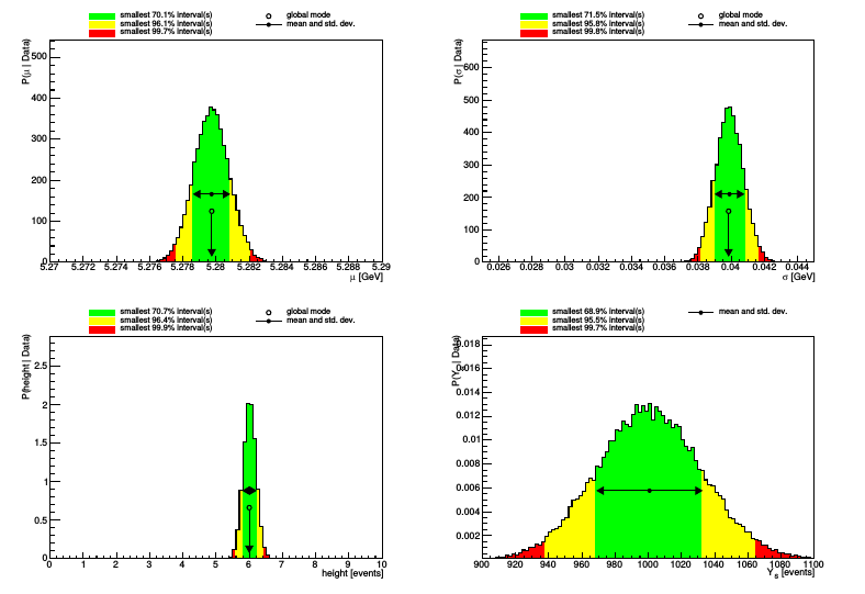
\
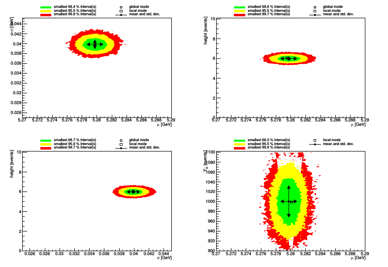
\
In each plot, we see the global mode and the marginalized mean and standard deviation of the posterior distribution; and three credibility intervals.
BAT has also printed a summary of the results to the log file and command line. This includes the global mode
Summary :  Global mode:
Summary :  0)  Parameter "mu"          : 5.279741 +- 0.001072076
Summary :  1)  Parameter "sigma"       : 0.040267 +- 0.00089553
Summary :  2)  Parameter "height"      : 6 +- 0.1897
and marginalized posteriors:
Summary :   (0) Parameter "mu" :
Summary :       Mean +- sqrt(Variance):         5.279748 +- 0.001065279
Summary :       Median +- central 68% interval: 5.279749 +  0.00105881 - -0.00106418
Summary :       (Marginalized) mode:            5.2797
Summary :        5% quantile:                   5.278005
Summary :       10% quantile:                   5.278381
Summary :       16% quantile:                   5.278685
Summary :       84% quantile:                   5.280808
Summary :       90% quantile:                   5.281112
Summary :       95% quantile:                   5.281498
Summary :       Smallest interval containing 69.8% and local mode:
Summary :       (5.2786, 5.2808) (local mode at 5.2797 with rel. height 1; rel. area 1)
Adding an observable
We can store the posterior distribution of any function of the parameters of our model using BAT's BCObservable's. Let us suppose we want to know the posterior distribution for the total number of events our model predicts—the signal yield; and we want to know the standard deviation's relation to the mean: \(\sigma/\mu\). In our constructor, we add the observables in the same way we added our parameters:
Note that an observable does not need a prior since it is not a parameter; but it does need a range for setting the marginalized histogram's limits. Since we know already that the answer will be 1000 events with an uncertainty of \(\sqrt{1000}\), we set the range for the yield to \([900, 1100]\).
And we need to calculate this observable in our CalculateObservables(...) member function. Uncomment it in the header file MyMod.h:
and implement it in the source:
Compile and run runMyTut.cxx and you will see new marginalized distributions and text output for the observables:
Summary :   (3) Observable "SignalYield" :
Summary :       Mean +- sqrt(Variance):         1000.9 +- 31.53
Summary :       Median +- central 68% interval: 1000.6 +  31.937 - -31.194
Summary :       (Marginalized) mode:            1003
Summary :        5% quantile:                   949.52
Summary :       10% quantile:                   960.52
Summary :       16% quantile:                   969.44
Summary :       84% quantile:                   1032.6
Summary :       90% quantile:                   1041.9
Summary :       95% quantile:                   1053.5
Summary :       Smallest intervals containing 68.7% and local modes:
Summary :       (970, 1032) (local mode at 1003 with rel. height 1; rel. area 0.97769)
Summary :       (1032, 1034) (local mode at 1033 with rel. height 0.57407; rel. area 0.022311)
As we expected, the mean of the total yield posterior is just the number of events in our data set and the standard deviation is its square root.
Further Output
BAT has a few more output options than the two mentioned above. The code for turning them on is already included in the runMyTut.cxx generated by bat-project. You can write the Markov-chain samples to a ROOT TTree for further postprocessing by uncommenting the following line:
You can also modify the plotting output to include more plots per page. Without specifying, we used the default of one plot per page. Let's instead plot 4 plots (in a 2-by-2 grid):
There are four more graphical outputs from BAT. Turn them on by uncommenting the following lines
(We have edited the last line to specify 3-by-2 printing.)
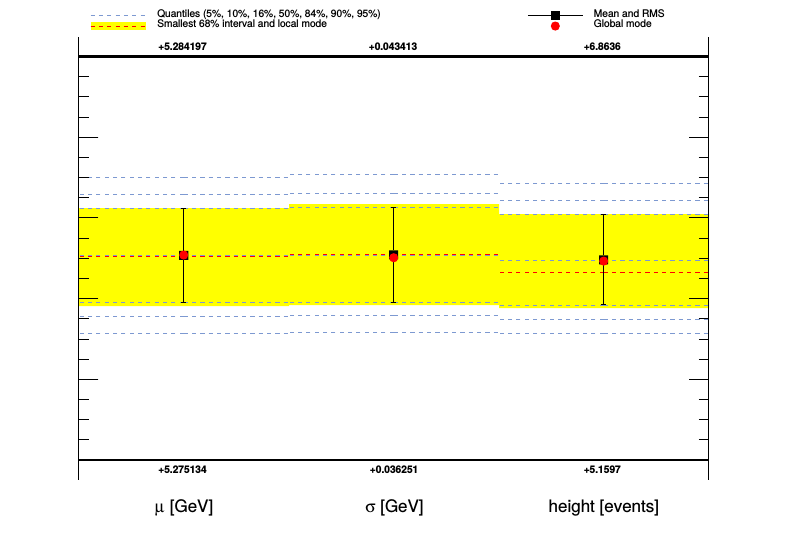
The parameter plot graphically summarizes the output for all parameters (and in a separate page, all observables) in a single image:
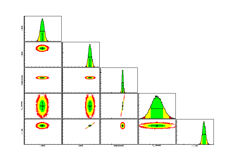
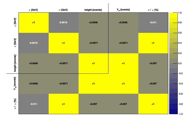
The correlation plot and the correlation matrix summarize graphically the correlations among parameters and observables:
The knowledge update plots show the marginalized priors and marginalized posteriors together in one plot for each variable (and also for 2D marginalizations):
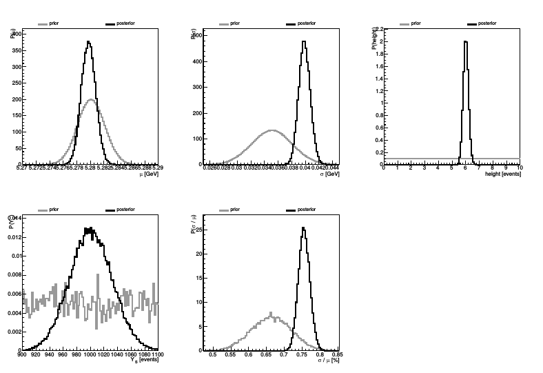
Note that this really shows the marginalized prior: Here, having used factorized priors, we see exactly the factorized priors. But had we used a multivariate prior, then we'd see what this looks like for each parameter. We also see what the prior of our observables look like given the priors of the variables they are functions of. These are very useful things to know.