Astro Imaging Example

You can also download this example as a Jupyter notebook and a plain Julia source file.

Introduction

In this example we reconstruct a simulated astronomical image from photon counts. The sky model has two components: diffuse emission (dust, nebulae) with unknown brightness, contrast and correlation structure, and point-like stars that can outshine the diffuse background in single pixels. Each pixel of the simulated detector records Poisson-distributed counts, and MGVI fits both components jointly.

Prepare the environment

using MGVI

using Distributions
using FFTW
using Random
using Statistics
using Plots
using ForwardDiffPullbacks

import ForwardDiff, Zygote
import DistributionsAD # provides the AD rules Zygote needs for Distributions
using AutoDiffOperators

context = MGVIContext(ADSelector(Zygote))

Plots.default(dpi=120, size=(600, 500))

Random.seed!(122);

The sky model

The detector image spans data_dim pixels. The diffuse emission is modeled on a pad_factor times larger grid, so that the periodic boundary conditions of its Fourier-space representation cannot fold emission from one image edge into the opposite one. A SkyModel object carries the grid sizes and the harmonic wave numbers k of the modeling grid, everything else is derived from them:

struct SkyModel <: Function
    data_dim::NTuple{2,Int}
    gp_dim::NTuple{2,Int}
    k::Matrix{Float64}
    k_ref::Float64
end

function SkyModel(; data_dim::NTuple{2,<:Integer}, pad_factor::Integer = 2)
    gp_dim = pad_factor .* data_dim
    kfreq(n) = [(i <= n ÷ 2 ? i : i - n) / n for i in 0:(n - 1)]
    k = hypot.(kfreq(gp_dim[1]), permutedims(kfreq(gp_dim[2])))
    SkyModel(data_dim, gp_dim, k, 1 / maximum(gp_dim))
end;

MGVI models map a flat vector p of parameters with standard normal priors to a distribution of the data. The first three entries of p are the hyperparameters of the diffuse emission, followed by one latent parameter per modeling grid cell for the diffuse emission and one parameter per image pixel for the stars:

hyper_idxs(::SkyModel) = 1:3
gp_idxs(m::SkyModel) = (1:prod(m.gp_dim)) .+ last(hyper_idxs(m))
star_idxs(m::SkyModel) = (1:prod(m.data_dim)) .+ last(gp_idxs(m))
n_params(m::SkyModel) = last(star_idxs(m));

The image pixels form the central block of the padded modeling grid:

data_idxs(m::SkyModel) = map((o, n) -> (o + 1):(o + n), (m.gp_dim .- m.data_dim) .÷ 2, m.data_dim);

Harmonic transform

As harmonic transform we choose the discrete Hartley transform (DHT), which maps real-valued functions to real-valued harmonic coefficients and is its own inverse up to a factor of the grid size. We compute it via a complex FFT as real(F) - imag(F): unlike FFTW's real-to-real plans, this composes with automatic differentiation and program tracing, and it generalizes correctly to multiple dimensions (the two-dimensional Hartley kernel is not the product of two one-dimensional ones):

function dht(x::AbstractArray)
    F = fft(Complex.(x))
    return real.(F) .- imag.(F)
end;

Reverse-mode AD handles dht out of the box. For forward-mode AD (MGVI uses it for Jacobian-vector products) we exploit that the DHT is linear, so it transforms dual values and partial derivatives independently:

function dht(x::AbstractArray{ForwardDiff.Dual{T,V,N}}) where {T,V,N}
    val = dht(ForwardDiff.value.(x))
    parts = ntuple(i -> dht(ForwardDiff.partials.(x, i)), Val(N))
    return ForwardDiff.Dual{T}.(val, parts...)
end;

Emission components

The log-brightness of the diffuse emission is a Gaussian random field with a power-law amplitude spectrum A(k) ∝ k^-α. Its three hyperparameters — mean log-brightness offset, contrast fluctuations and spectral slope α — have standard normal priors like all other parameters, so they are rescaled to their intended ranges inside the model. The amplitude spectrum is normalized such that fluctuations directly gives the a priori standard deviation of the log-brightness:

function diffuse_emission(m::SkyModel, p::AbstractVector)
    ξ_offset, ξ_fluct, ξ_slope = p[hyper_idxs(m)]
    offset = log(3.0) + 1.0 * ξ_offset
    fluctuations = 1.5 * exp(0.3 * ξ_fluct)
    α = 1.5 + 0.25 * ξ_slope
    k_safe = ifelse.(m.k .== 0, one.(m.k), m.k)
    A_raw = ifelse.(m.k .== 0, zero(α), (k_safe ./ m.k_ref) .^ -α)
    A = fluctuations .* A_raw ./ sqrt(sum(abs2, A_raw) / length(A_raw))
    ξ_gp = reshape(p[gp_idxs(m)], m.gp_dim)
    log_brightness = offset .+ dht(A .* ξ_gp) ./ sqrt(prod(m.gp_dim))
    exp.(log_brightness[data_idxs(m)...])
end;

Stars are point-like, so they need no correlation structure: each image pixel gets an independent star brightness with a heavy-tailed log-normal prior. Most pixels stay dark, but dozens of the brightest ones a priori host stars that outshine the diffuse emission:

function star_emission(m::SkyModel, p::AbstractVector)
    exp.(-6.5 .+ 3.2 .* reshape(p[star_idxs(m)], m.data_dim))
end;

total_emission(m::SkyModel, p::AbstractVector) = diffuse_emission(m, p) .+ star_emission(m, p);

Each pixel records counts drawn from a Poisson distribution with the total emission as rate. Wrapping the Poisson constructor via fwddiff from ForwardDiffPullbacks makes the broadcast efficient for reverse-mode AD:

function (m::SkyModel)(p::AbstractVector)
    product_distribution(fwddiff(Poisson).(vec(total_emission(m, p))))
end;

Simulated data

We instantiate the sky model and draw the ground truth from the prior:

sky = SkyModel(data_dim = (96, 96))

true_params = randn(n_params(sky));
data = rand(sky(true_params));

plot(
    heatmap(diffuse_emission(sky, true_params), title="true diffuse emission"),
    heatmap(star_emission(sky, true_params), title="true stars"),
    heatmap(log10.(total_emission(sky, true_params)), title="true total emission (log10)"),
    heatmap(log10.(reshape(data, sky.data_dim) .+ 1), title="observed counts (log10(1+n))"),
    layout=(2, 2), size=(900, 700)
)
savefig("astro-img-plot1.png")

"/home/runner/work/MGVI.jl/MGVI.jl/docs/build/astro-img-plot1.png"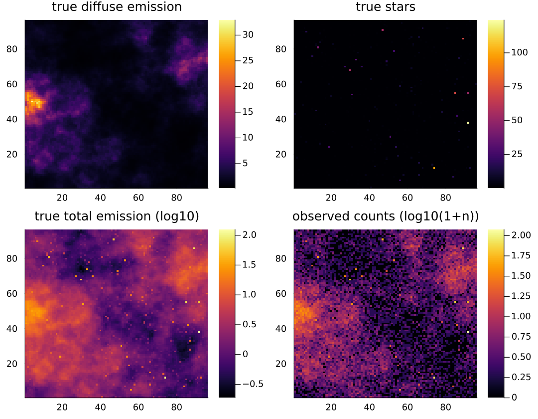

Fitting

We prepare the MGVI step once for the model, data and parameter size, and then iterate it, starting from the prior mean. Preparation makes repeated steps cheap, and for accelerator devices (via the device keyword of mgvi_prepare) the prepared step can even be compiled into a single device program. Each step draws new residual samples around the current parameter estimate, so the mean negative log-posterior mnlp fluctuates slightly even after convergence:

config = MGVIConfig(
    linsolver_opts = (;maxiters = 30),
    optimizer = MGVI.NewtonCG(steps = 3, cg_maxiter = 20)
)

center = zeros(n_params(sky))
prepared = mgvi_prepare(sky, data, 4, center, config, context)

mnlp_series = Float64[]
result = nothing
for i in 1:12
    global result, center = mgvi_step(prepared, center)
    push!(mnlp_series, result.mnlp)
end

plot(mnlp_series, yscale=:log10, marker=:circle, label="mnlp", xlabel="iteration")
savefig("astro-img-plot2.pdf")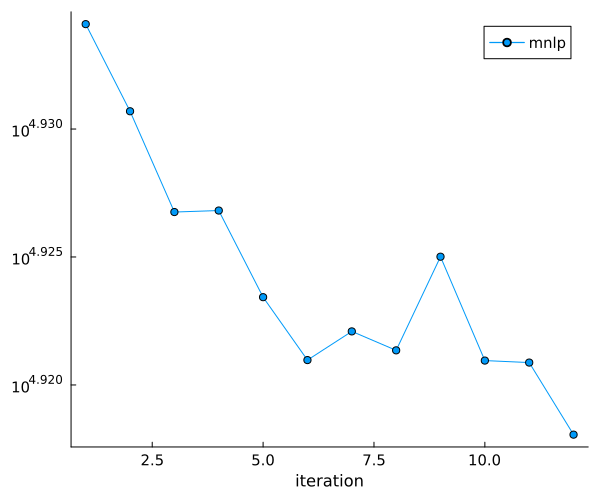

Results

The reconstruction separates the two components: the diffuse emission is recovered as a smooth field, and the bright stars are absorbed by the point-source component instead of leaving imprints in the diffuse map:

plot(
    heatmap(diffuse_emission(sky, true_params), title="true diffuse emission"),
    heatmap(diffuse_emission(sky, center), title="reconstructed diffuse emission"),
    heatmap(star_emission(sky, true_params), title="true stars"),
    heatmap(star_emission(sky, center), title="reconstructed stars"),
    layout=(2, 2), size=(900, 700)
)
savefig("astro-img-plot3.png")

"/home/runner/work/MGVI.jl/MGVI.jl/docs/build/astro-img-plot3.png"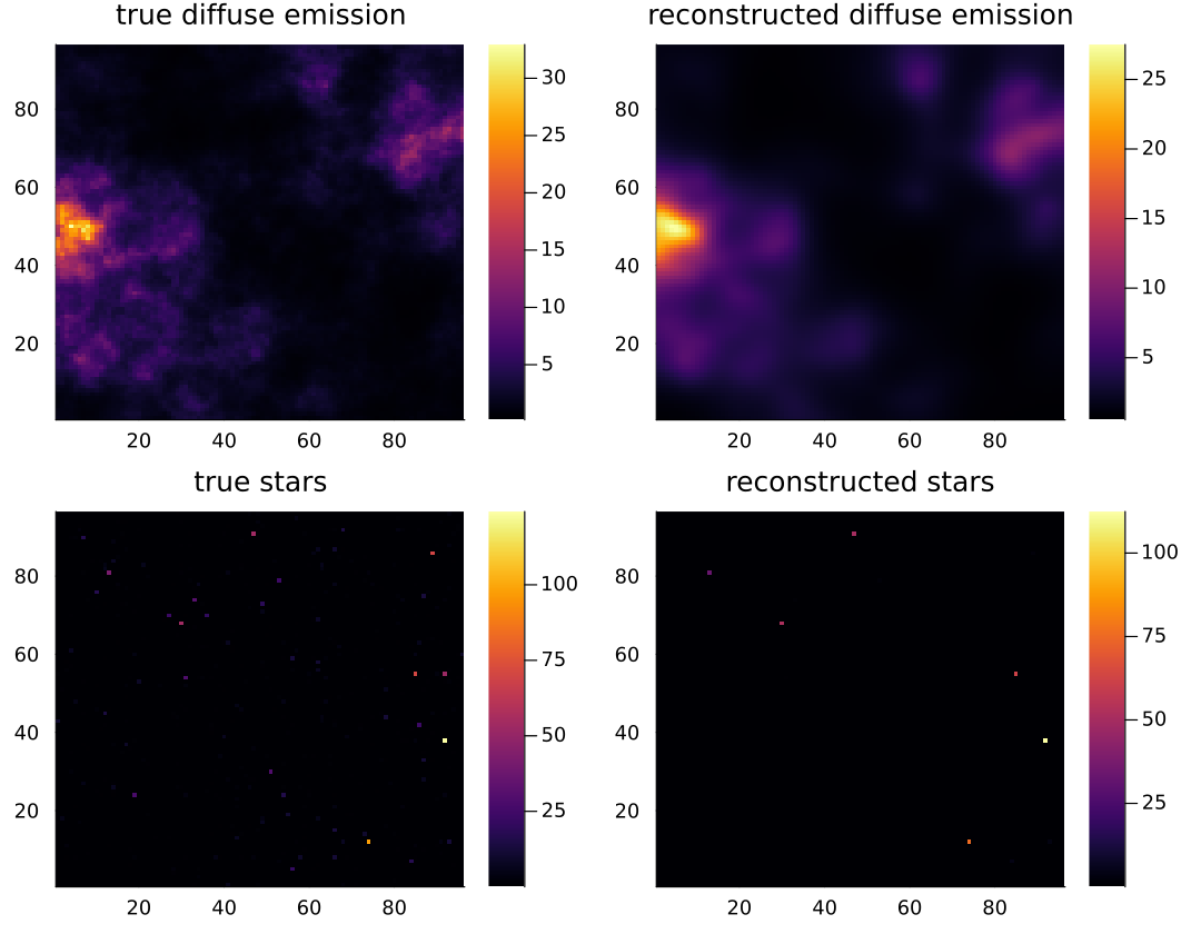

The brightness of the reconstructed stars closely follows the truth for stars that stand out of the diffuse background, while stars fainter than the background are only weakly constrained by the data:

star_sel = findall(vec(star_emission(sky, true_params)) .> 1);

scatter(
    vec(star_emission(sky, true_params))[star_sel], vec(star_emission(sky, center))[star_sel],
    xscale=:log10, yscale=:log10, xlabel="true star brightness",
    ylabel="reconstructed star brightness", label=nothing
)
plot!(identity, label="truth")
savefig("astro-img-plot4.pdf")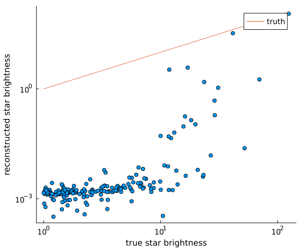

MGVI approximates the posterior by a Gaussian in the standardized parameters, centered on the final parameter estimate with the inverse Fisher metric as covariance. Samples from this posterior approximation can be drawn at any time via MGVI.sample_residuals, as antithetic pairs center ± residual:

residuals = MGVI.sample_residuals(
    sky, center,
    randn(prod(sky.data_dim), 16), randn(n_params(sky), 16),
    context.ad
);
post_samples = hcat(center .+ residuals, center .- residuals);

Per-pixel standard deviations of the log-brightness over the posterior samples provide an uncertainty map of the reconstruction: the emission is tightly constrained where it is bright, while for dark pixels the data only provide upper limits on a possible star, so the uncertainty is dominated by the star prior there:

sample_log_emissions = [log10.(total_emission(sky, Vector(s))) for s in eachcol(post_samples)];

plot(
    heatmap(log10.(total_emission(sky, center)), title="reconstructed total emission (log10)"),
    heatmap(std(sample_log_emissions), title="posterior uncertainty (dex)"),
    layout=(1, 2), size=(900, 350)
)
savefig("astro-img-plot5.png")

"/home/runner/work/MGVI.jl/MGVI.jl/docs/build/astro-img-plot5.png"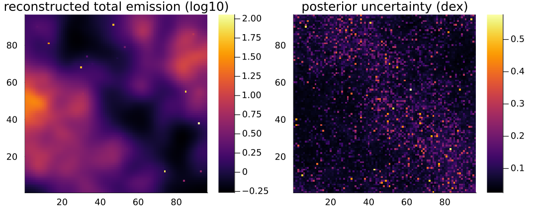

This page was generated using Literate.jl.