Tutorial

This tutorial demonstrates a simple application of BAT.jl: A Bayesian fit of a histogram with two Gaussian peaks.

You can also download this tutorial as a Jupyter notebook and a plain Julia source file.

Table of contents:

• Tutorial
• • Input Data Generation
  • Bayesian Fit
  • • Likelihood Definition
    • Prior Definition
    • Bayesian Model Definition
    • Parameter Space Exploration via MCMC
    • Visualization of Results
    • Integration with Tables.jl
  • Comparison of Truth and Best Fit
  • Fine-grained control
  • Saving result data to files

Note: This tutorial is somewhat verbose, as it aims to be easy to follow for users who are new to Julia. For the same reason, we deliberately avoid making use of Julia features like closures, anonymous functions, broadcasting syntax, performance annotations, etc.

Input Data Generation

First, let's generate some synthetic data to fit. We'll need the Julia standard-library packages "Random", "LinearAlgebra" and "Statistics", as well as the packages "Distributions" and "StatsBase":

using Random, LinearAlgebra, Statistics, Distributions, StatsBase

As the underlying truth of our input data/histogram, let us choose the expected count to follow the sum of two Gaussian peaks with peak areas of 500 and 1000, a mean of -1.0 and 2.0 and a standard error of 0.5. Then

data = vcat(
    rand(Normal(-1.0, 0.5), 500),
    rand(Normal( 2.0, 0.5), 1000)
)

1500-element Vector{Float64}:
 -1.4778384723249147
 -0.8029919003598135
 -0.6629532391322672
 -1.4340931011598044
 -1.4439445974301033
 -0.7834303712276468
 -1.3662579408961077
 -0.2399561340346008
 -1.5807174869083702
 -1.18917614520168
  ⋮
  2.12566366941473
  0.6344586109201569
  1.7954538863458067
  1.5625961359270655
  1.802340476564834
  1.3944530496979868
  1.7817543505167774
  1.7098975505142984
  1.6940630858188572

resulting in a vector of floating-point numbers:

typeof(data) == Vector{Float64}

true

Next, we'll create a histogram of that data, this histogram will serve as the input for the Bayesian fit:

hist = append!(Histogram(-2:0.1:4), data)

StatsBase.Histogram{Int64, 1, Tuple{StepRangeLen{Float64, Base.TwicePrecision{Float64}, Base.TwicePrecision{Float64}, Int64}}}
edges:
  -2.0:0.1:4.0
weights: [4, 9, 12, 23, 26, 33, 33, 37, 33, 40  …  7, 4, 0, 5, 1, 0, 0, 0, 0, 0]
closed: left
isdensity: false

Using the Julia "Plots" package

using Plots

we can plot the histogram:

plot(
    normalize(hist, mode=:density),
    st = :steps, label = "Data",
    title = "Data"
)
savefig("tutorial-data.pdf")

Let's define our fit function - the function that we expect to describe the data histogram, at each x-Axis position x, depending on a given set p of model parameters:

function fit_function(p::NamedTuple{(:a, :mu, :sigma)}, x::Real)
    p.a[1] * pdf(Normal(p.mu[1], p.sigma), x) +
    p.a[2] * pdf(Normal(p.mu[2], p.sigma), x)
end

The fit parameters (model parameters) a (peak areas) and mu (peak means) are vectors, parameter sigma (peak width) is a scalar, we assume it's the same for both Gaussian peaks.

The true values for the model/fit parameters are the values we used to generate the data:

true_par_values = (a = [500, 1000], mu = [-1.0, 2.0], sigma = 0.5)

Let's visually compare the histogram and the fit function, using these true parameter values, to make sure everything is set up correctly:

plot(
    normalize(hist, mode=:density),
    st = :steps, label = "Data",
    title = "Data and True Statistical Model"
)
plot!(
    -4:0.01:4, x -> fit_function(true_par_values, x),
    label = "Truth"
)
savefig("tutorial-data-and-truth.pdf")

Bayesian Fit

Now we'll perform a Bayesian fit of the generated histogram, using BAT, to infer the model parameters from the data histogram.

In addition to the Julia packages loaded above, we need BAT itself, as well as IntervalSets:

using BAT, DensityInterface, IntervalSets

Likelihood Definition

First, we need to define the likelihood (function) for our problem.

BAT represents densities like likelihoods and priors as subtypes of BAT.AbstractMeasureOrDensity. Custom likelihood can be defined by creating a new subtype of AbstractMeasureOrDensity and by implementing (at minimum) DensityInterface.logdensityof for that type - in complex uses cases, this may become necessary. Typically, however, it is sufficient to define a custom likelihood as a simple function that returns the log-likelihood value for a given set of parameters. BAT will automatically convert such a likelihood function into a subtype of AbstractMeasureOrDensity.

For performance reasons, functions should not access global variables directly. So we'll use an anonymous function inside of a let-statement to capture the value of the global variable hist in a local variable h (and to shorten function name fit_function to f, purely for convenience). DensityInterface.logfuncdensity turns a log-likelihood function into a density object.

likelihood = let h = hist, f = fit_function
    # Histogram counts for each bin as an array:
    observed_counts = h.weights

    # Histogram binning:
    bin_edges = h.edges[1]
    bin_edges_left = bin_edges[1:end-1]
    bin_edges_right = bin_edges[2:end]
    bin_widths = bin_edges_right - bin_edges_left
    bin_centers = (bin_edges_right + bin_edges_left) / 2

    logfuncdensity(function (params)
        # Log-likelihood for a single bin:
        function bin_log_likelihood(i)
            # Simple mid-point rule integration of fit function `f` over bin:
            expected_counts = bin_widths[i] * f(params, bin_centers[i])
            # Avoid zero expected counts for numerical stability:
            logpdf(Poisson(expected_counts + eps(expected_counts)), observed_counts[i])
        end

        # Sum log-likelihood over bins:
        idxs = eachindex(observed_counts)
        ll_value = bin_log_likelihood(idxs[1])
        for i in idxs[2:end]
            ll_value += bin_log_likelihood(i)
        end

        return ll_value
    end)
end

LogFuncDensity(Main.var"#3#4"{StepRangeLen{Float64, Base.TwicePrecision{Float64}, Base.TwicePrecision{Float64}, Int64}, StepRangeLen{Float64, Base.TwicePrecision{Float64}, Base.TwicePrecision{Float64}, Int64}, Vector{Int64}, typeof(Main.fit_function)}(-1.95:0.1:3.95, StepRangeLen(0.1, 0.0, 60), [4, 9, 12, 23, 26, 33, 33, 37, 33, 40  …  7, 4, 0, 5, 1, 0, 0, 0, 0, 0], Main.fit_function))

BAT makes use of Julia's parallel programming facilities if possible, e.g. to run multiple Markov chains in parallel. Therefore, log-likelihood (and other) code must be thread-safe. Mark non-thread-safe code with @critical (provided by Julia package ParallelProcessingTools).

Support for automatic parallelization across multiple (local and remote) Julia processes is planned, but not implemented yet.

Note that Julia currently starts only a single thread by default. Set the the environment variable JULIA_NUM_THREADS to specify the desired number of Julia threads.

We can evaluate likelihood, e.g. at the true parameter values:

logdensityof(likelihood, true_par_values)

-156.47960338983776

Prior Definition

Next, we need to choose a sensible prior for the fit:

prior = distprod(
    a = [Weibull(1.1, 5000), Weibull(1.1, 5000)],
    mu = [-2.0..0.0, 1.0..3.0],
    sigma = Weibull(1.2, 2)
)

In general, BAT allows instances of any subtype of AbstractMeasureOrDensity to be uses as a prior, as long as a sampler is defined for it. This way, users may implement complex application-specific priors. You can also use convert(AbstractMeasureOrDensity, distribution) to convert any continuous multivariate Distributions.Distribution to a BAT.AbstractMeasureOrDensity that can be used as a prior (or likelihood).

Bayesian Model Definition

Given the likelihood and prior definition, a BAT.PosteriorMeasure is simply defined via

posterior = PosteriorMeasure(likelihood, prior)

Parameter Space Exploration via MCMC

We can now use Markov chain Monte Carlo (MCMC) to explore the space of possible parameter values for the histogram fit.

To increase the verbosity level of BAT logging output, you may want to set the Julia logging level for BAT to debug via ENV["JULIA_DEBUG"] = "BAT".

Now we can generate a set of MCMC samples via bat_sample. We'll use 4 MCMC chains with 10^5 MC steps in each chain (after tuning/burn-in):

samples = bat_sample(posterior, MCMCSampling(mcalg = MetropolisHastings(), nsteps = 10^5, nchains = 4)).result

[ Info: Setting new default BAT context BATContext{Float64}(Random123.Philox4x{UInt64, 10}(0x2a9cb5cf90a99b44, 0xc1f7814437ffa7d0, 0xc8df551cbbdd0e62, 0x044af0863ad11e9c, 0x9704e315742ee1ae, 0x1deb6f80ee3b81f2, 0x0000000000000000, 0x0000000000000000, 0x0000000000000000, 0x0000000000000000, 0), HeterogeneousComputing.CPUnit(), BAT._NoADSelected())
[ Info: MCMCChainPoolInit: trying to generate 4 viable MCMC chain(s).
[ Info: Selected 4 MCMC chain(s).
[ Info: Begin tuning of 4 MCMC chain(s).
[ Info: MCMC Tuning cycle 1 finished, 4 chains, 0 tuned, 0 converged.
[ Info: MCMC Tuning cycle 2 finished, 4 chains, 0 tuned, 0 converged.
[ Info: MCMC Tuning cycle 3 finished, 4 chains, 0 tuned, 0 converged.
[ Info: MCMC Tuning cycle 4 finished, 4 chains, 0 tuned, 0 converged.
[ Info: MCMC Tuning cycle 5 finished, 4 chains, 0 tuned, 4 converged.
[ Info: MCMC Tuning cycle 6 finished, 4 chains, 0 tuned, 4 converged.
[ Info: MCMC Tuning cycle 7 finished, 4 chains, 1 tuned, 4 converged.
[ Info: MCMC Tuning cycle 8 finished, 4 chains, 3 tuned, 4 converged.
[ Info: MCMC Tuning cycle 9 finished, 4 chains, 3 tuned, 4 converged.
[ Info: MCMC Tuning cycle 10 finished, 4 chains, 3 tuned, 4 converged.
[ Info: MCMC Tuning cycle 11 finished, 4 chains, 4 tuned, 4 converged.
[ Info: MCMC tuning of 4 chains successful after 11 cycle(s).
[ Info: Running post-tuning stabilization steps for 4 MCMC chain(s).

Let's calculate some statistics on the posterior samples:

println("Truth: $true_par_values")
println("Mode: $(mode(samples))")
println("Mean: $(mean(samples))")
println("Stddev: $(std(samples))")

Truth: (a = [500, 1000], mu = [-1.0, 2.0], sigma = 0.5)
Mode: (a = [495.06513020444606, 995.6297404430102], mu = [-1.032188633594704, 2.023260184346153], sigma = 0.4778842348756829)
Mean: (a = [498.9333824585944, 998.7589585614431], mu = [-1.0328324464106196, 2.023423624878714], sigma = 0.4794909862711996)
Stddev: (a = [22.673803343506727, 31.542766662164457], mu = [0.023510069379151607, 0.015315474969878213], sigma = 0.009335110880434119)

Internally, BAT often needs to represent variates as flat real-valued vectors:

unshaped_samples, f_flatten = bat_transform(Vector, samples)

(result = DensitySampleVector(length = 117497, varshape = ValueShapes.ArrayShape{Float64, 1}((5,))), trafo = Base.Fix2{typeof(ValueShapes.unshaped), ValueShapes.NamedTupleShape{(:a, :mu, :sigma), Tuple{ValueShapes.ValueAccessor{ValueShapes.ArrayShape{Real, 1}}, ValueShapes.ValueAccessor{ValueShapes.ArrayShape{Real, 1}}, ValueShapes.ValueAccessor{ValueShapes.ScalarShape{Real}}}, NamedTuple}}(ValueShapes.unshaped, NamedTupleShape((a = ValueShapes.ArrayShape{Real, 1}((2,)), mu = ValueShapes.ArrayShape{Real, 1}((2,)), sigma = ValueShapes.ScalarShape{Real}()))), optargs = (algorithm = BAT.UnshapeTransformation(), context = BATContext{Float64}(Random123.Philox4x{UInt64, 10}(0xf5a4242a2a96ff13, 0x11d2eba3ef578bff, 0xe320e669e5c8f41a, 0x4078961c31f2c51f, 0x9704e315742ee1ae, 0x1deb6f80ee3b81f2, 0x0000000000000000, 0x0000000000000000, 0x0000000000000000, 0x8000020100000000, 0), HeterogeneousComputing.CPUnit(), BAT._NoADSelected())))

The statisics above (mode, mean and std-dev) are presented in shaped form. However, it's not possible to represent statistics with matrix shape, e.g. the parameter covariance matrix, this way. So the covariance has to be accessed in unshaped form:

par_cov = cov(unshaped_samples)
println("Covariance: $par_cov")

Covariance: [514.1013580600173 -12.163243527031801 -0.04055224555364897 -0.0014560638539045576 0.013206374605210834; -12.163243527031801 994.9461287037457 -0.008488630580893967 -0.006724886727461252 0.002622759790724551; -0.04055224555364897 -0.008488630580893967 0.0005527233622125284 4.8215042004040825e-6 -2.950338800785283e-5; -0.0014560638539045576 -0.006724886727461252 4.8215042004040825e-6 0.00023456377355296764 -6.85051016177336e-7; 0.013206374605210834 0.002622759790724551 -2.950338800785283e-5 -6.85051016177336e-7 8.714429514999989e-5]

Use bat_report to generate an overview of the sampling result and parameter estimates (based on the marginal distributions):

bat_report(samples)

Visualization of Results

BAT.jl comes with an extensive set of plotting recipes for "Plots.jl". We can plot the marginalized distribution for a single parameter (e.g. parameter 3, i.e. μ[1]):

plot(
    samples, :(mu[1]),
    mean = true, std = true, globalmode = true, marginalmode = true,
    nbins = 50, title = "Marginalized Distribution for mu[1]"
)
savefig("tutorial-single-par.pdf")

or plot the marginalized distribution for a pair of parameters (e.g. parameters 3 and 5, i.e. μ[1] and σ), including information from the parameter stats:

plot(
    samples, (:(mu[1]), :sigma),
    mean = true, std = true, globalmode = true, marginalmode = true,
    nbins = 50, title = "Marginalized Distribution for mu[1] and sigma"
)
plot!(BAT.MCMCBasicStats(samples), (3, 5))
savefig("tutorial-param-pair.png")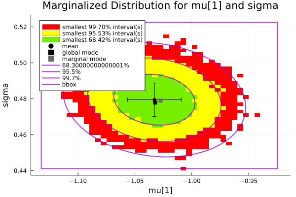

We can also create an overview plot of the marginalized distribution for all pairs of parameters:

plot(
    samples,
    mean = false, std = false, globalmode = true, marginalmode = false,
    nbins = 50
)
savefig("tutorial-all-params.png")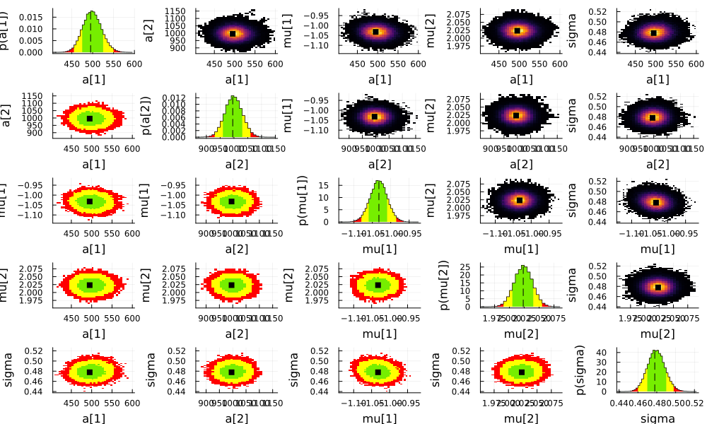

Integration with Tables.jl

DensitySamplesVector supports the Tables.jl interface, so it is a table itself. We can also convert it to other table types, e.g. a TypedTables.Table:

using TypedTables

tbl = Table(samples)

Table with 5 columns and 117497 rows:
      v                       logd      weight  info                    aux
    ┌──────────────────────────────────────────────────────────────────────────
 1  │ (a = [490.572, 1023.6…  -173.428  9       MCMCSampleID(25, 14, …  nothing
 2  │ (a = [488.063, 1028.6…  -173.668  11      MCMCSampleID(25, 14, …  nothing
 3  │ (a = [487.371, 1026.8…  -173.391  8       MCMCSampleID(25, 14, …  nothing
 4  │ (a = [500.078, 1019.9…  -174.534  2       MCMCSampleID(25, 14, …  nothing
 5  │ (a = [506.989, 1022.6…  -174.223  14      MCMCSampleID(25, 14, …  nothing
 6  │ (a = [504.523, 1023.6…  -173.691  7       MCMCSampleID(25, 14, …  nothing
 7  │ (a = [495.593, 1028.6…  -174.898  5       MCMCSampleID(25, 14, …  nothing
 8  │ (a = [492.109, 1026.6…  -175.45   4       MCMCSampleID(25, 14, …  nothing
 9  │ (a = [505.664, 1017.9…  -174.904  1       MCMCSampleID(25, 14, …  nothing
 10 │ (a = [500.003, 1023.3…  -175.017  6       MCMCSampleID(25, 14, …  nothing
 11 │ (a = [489.07, 1030.82…  -177.438  7       MCMCSampleID(25, 14, …  nothing
 12 │ (a = [496.665, 1028.7…  -174.437  3       MCMCSampleID(25, 14, …  nothing
 13 │ (a = [504.085, 1016.7…  -174.724  1       MCMCSampleID(25, 14, …  nothing
 14 │ (a = [503.685, 1023.5…  -173.813  5       MCMCSampleID(25, 14, …  nothing
 15 │ (a = [515.573, 1025.3…  -173.477  7       MCMCSampleID(25, 14, …  nothing
 16 │ (a = [513.079, 1032.9…  -173.331  2       MCMCSampleID(25, 14, …  nothing
 17 │ (a = [514.495, 1037.0…  -173.329  2       MCMCSampleID(25, 14, …  nothing
 ⋮  │           ⋮                ⋮        ⋮               ⋮                ⋮

or a DataFrames.DataFrame, etc.

Comparison of Truth and Best Fit

As a final step, we retrieve the parameter values at the mode, representing the best-fit parameters

samples_mode = mode(samples)

(a = [495.06513020444606, 995.6297404430102], mu = [-1.032188633594704, 2.023260184346153], sigma = 0.4778842348756829)

Like the samples themselves, the result can be viewed in both shaped and unshaped form. samples_mode is presented as a 0-dimensional array that contains a NamedTuple, this representation preserves the shape information:

samples_mode isa NamedTuple

true

samples_mode is only an estimate of the mode of the posterior distribution. It can be further refined using bat_findmode:

using Optim

findmode_result = bat_findmode(
    posterior,
    OptimAlg(optalg = Optim.NelderMead(), init = ExplicitInit([samples_mode]))
)

fit_par_values = findmode_result.result

(a = [497.9244011224433, 998.6812937696279], mu = [-1.0321842572862276, 2.023547582313582], sigma = 0.4787080426855382)

Let's plot the data and fit function given the true parameters and MCMC samples

plot(-4:0.01:4, fit_function, samples)

plot!(
    normalize(hist, mode=:density),
    color=1, linewidth=2, fillalpha=0.0,
    st = :steps, fill=false, label = "Data",
    title = "Data, True Model and Best Fit"
)

plot!(-4:0.01:4, x -> fit_function(true_par_values, x), color=4, label = "Truth")
savefig("tutorial-data-truth-bestfit.pdf")

Fine-grained control

BAT provides fine-grained control over the MCMC algorithm options, the MCMC chain initialization, tuning/burn-in strategy and convergence testing. All option value used in the following are the default values, any or all may be omitted.

We'll sample using the The Metropolis-Hastings MCMC algorithm:

mcmcalgo = MetropolisHastings(
    weighting = RepetitionWeighting(),
    tuning = AdaptiveMHTuning()
)

MetropolisHastings{BAT.MvTDistProposal, RepetitionWeighting{Int64}, AdaptiveMHTuning}
  proposal: BAT.MvTDistProposal
  weighting: RepetitionWeighting{Int64} RepetitionWeighting{Int64}()
  tuning: AdaptiveMHTuning

BAT requires a counter-based random number generator (RNG), since it partitions the RNG space over the MCMC chains. This way, a single RNG seed is sufficient for all chains and results are reproducible even under parallel execution. By default, BAT uses a Philox4x RNG initialized with a random seed drawn from the system entropy pool:

using Random123
rng = Philox4x()
context = BATContext(rng = Philox4x())

By default, MetropolisHastings() uses the following options.

For Markov chain initialization:

init = MCMCChainPoolInit()

MCMCChainPoolInit
  init_tries_per_chain: IntervalSets.ClosedInterval{Int64}
  nsteps_init: Int64 1000
  initval_alg: InitFromTarget InitFromTarget()

For the MCMC burn-in procedure:

burnin = MCMCMultiCycleBurnin()

MCMCMultiCycleBurnin
  nsteps_per_cycle: Int64 10000
  max_ncycles: Int64 30
  nsteps_final: Int64 1000

For convergence testing:

convergence = BrooksGelmanConvergence()

BrooksGelmanConvergence
  threshold: Float64 1.1
  corrected: Bool false

To generate MCMC samples with explicit control over all options, use something like

samples = bat_sample(
    posterior,
    MCMCSampling(
        mcalg = mcmcalgo,
        nchains = 4,
        nsteps = 10^5,
        init = init,
        burnin = burnin,
        convergence = convergence,
        strict = true,
        store_burnin = false,
        nonzero_weights = true,
        callback = (x...) -> nothing
    ),
    context
).result

[ Info: MCMCChainPoolInit: trying to generate 4 viable MCMC chain(s).
[ Info: Selected 4 MCMC chain(s).
[ Info: Begin tuning of 4 MCMC chain(s).
[ Info: MCMC Tuning cycle 1 finished, 4 chains, 0 tuned, 0 converged.
[ Info: MCMC Tuning cycle 2 finished, 4 chains, 0 tuned, 0 converged.
[ Info: MCMC Tuning cycle 3 finished, 4 chains, 0 tuned, 0 converged.
[ Info: MCMC Tuning cycle 4 finished, 4 chains, 0 tuned, 0 converged.
[ Info: MCMC Tuning cycle 5 finished, 4 chains, 0 tuned, 4 converged.
[ Info: MCMC Tuning cycle 6 finished, 4 chains, 0 tuned, 4 converged.
[ Info: MCMC Tuning cycle 7 finished, 4 chains, 1 tuned, 4 converged.
[ Info: MCMC Tuning cycle 8 finished, 4 chains, 1 tuned, 4 converged.
[ Info: MCMC Tuning cycle 9 finished, 4 chains, 2 tuned, 4 converged.
[ Info: MCMC Tuning cycle 10 finished, 4 chains, 3 tuned, 4 converged.
[ Info: MCMC Tuning cycle 11 finished, 4 chains, 4 tuned, 4 converged.
[ Info: MCMC tuning of 4 chains successful after 11 cycle(s).
[ Info: Running post-tuning stabilization steps for 4 MCMC chain(s).

Saving result data to files

The package FileIO.jl(in conjunction with JLD2.jl) offers a convenient way to store results like posterior samples to file:

using FileIO
import JLD2
FileIO.save("results.jld2", Dict("samples" => samples))

JLD2 persists the full information (including value shapes), so you can reload exactly the same data into memory in a new Julia session via

using FileIO
import JLD2
samples = FileIO.load("results.jld2", "samples")

provided you use compatible versions of BAT and it's dependencies. Note that JLD2 is not a long-term stable file format. Also note that this functionality is provided by FileIO.jl and JLD2.jl and not part of the BAT API itself.

BAT.jl itself can write samples to standard HDF5 files in a form suitable for long-term storage (via HDF5.jl):

import HDF5
bat_write("results.h5", samples)

The resulting files have an intuitive HDF5 layout and can be read with the standard HDF5 libraries, so they are easily accessible from other programming languages as well. Not all value shape information can be preserved, though. To read BAT.jl HDF5 sample data, use

using BAT
import HDF5
samples = bat_read("results.h5").result

BAT.jl's HDF5 file format may evolve over time, but future versions of BAT.jl will be able to read HDF5 sample data written by this version of BAT.jl.

This page was generated using Literate.jl.